Predicting Weight Loss with Machine Learning

I’ve been writing on my blog about following a ketogenic diet to manage my mental illness – see Finding Hope After Decades of Struggle. One of the major wins I’ve been able to achieve so far is losing over 20 kg in the last couple of months.

I have been tracking my weight every week for about 8 weeks now and thought it would be interesting to implement a simple DNN machine learning model to fit that data and try to extrapolate my weight loss into the near future. After several iterations and adjustments, I worked with ChatGPT to generate this Python script to:

I chose to use a simple feedforward DNN model to capture the non-linear nature of the weight loss time series. I assumed a basic DNN model would be easy to implement, train, and fast in inference mode.

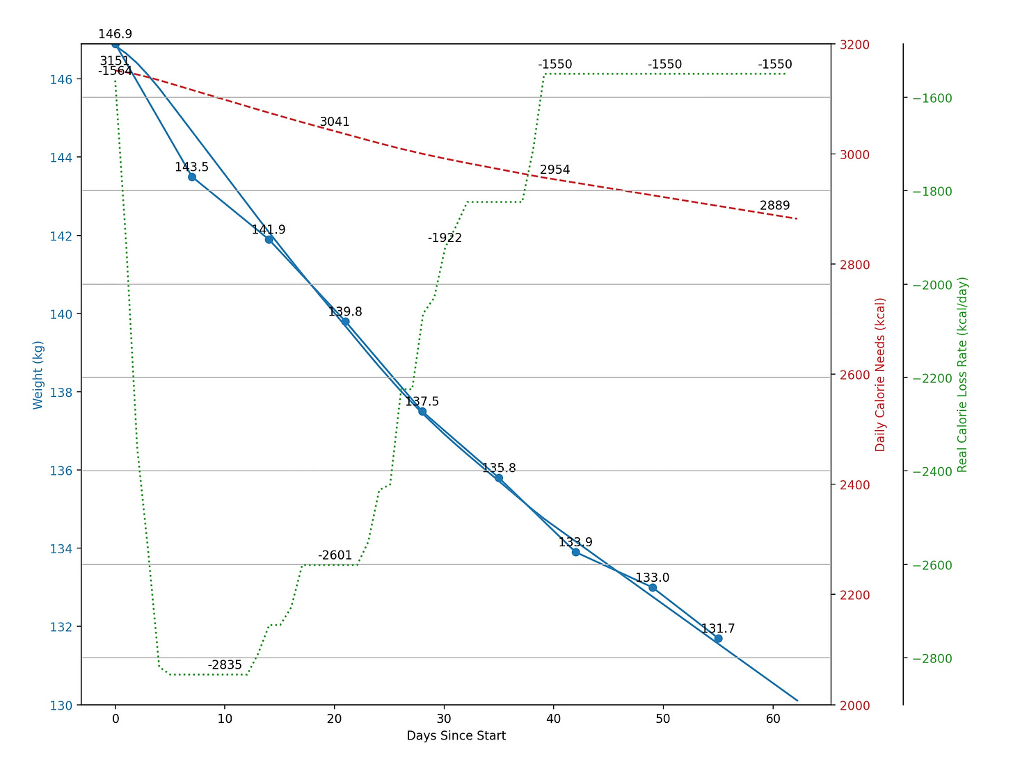
Additionally, I used the Harris-Benedict Equation to create a graph of the daily calorie needs required to maintain my weight at each point in the weight loss series. This graph can be compared to the real weight loss rate to understand how many calories I was below the maintenance level at each point:

The Harris-Benedict Equation, often referred to as the Harris weight loss function, is a well-established mathematical model used to estimate an individual’s Basal Metabolic Rate (BMR) and Total Daily Energy Expenditure (TDEE). BMR refers to the number of calories your body needs to perform basic physiological functions like breathing, circulation, and cell production when at rest. The equation also helps calculate how many calories you need to maintain your current weight and can be adjusted to estimate calorie needs for weight loss or gain.

Here’s a diagram of the simple feedforward DNN model:

And here’s the final graph showing the non-linear function fit to my weight loss series, along with two graphs tracking calorie metrics to better understand the metabolic dynamics behind the process:

There’s an initial large drop, followed by a gradual decrease and stabilization in my weekly calorie deficit after starting the ketogenic diet. Interestingly, the weight loss function shows a near-constant decrease rate throughout the process, even as my calorie restriction (relative to the calculated Harris-Benedict BMR and TDEE) seems to have stabilized at a level that keeps me feeling satisfied without much effort.

Below is the source code I used to generate the graphs (it can run on a regular CPU in about 30 seconds):

import os
import numpy as np
import pandas as pd
import tensorflow as tf
from sklearn.model_selection import train_test_split
from sklearn.preprocessing import MinMaxScaler
import matplotlib.pyplot as plt
from datetime import datetime, timedelta

# Disable GPU and force TensorFlow to use only the CPU
tf.config.set_visible_devices([], 'GPU')  # Disable GPU usage

# Harris-Benedict Equation for BMR (Male)
def harris_benedict_bmr(weight, height_cm, age, gender="male"):
    if gender is 'male':
        return 88.362 + (13.397 * weight) + (4.799 * height_cm) - (5.677 * age)
    else:
        return 447.593 + (9.247 * weight) + (3.098 * height_cm) - (4.330 * age)

# Activity factor (e.g., sedentary)
activity_factor = 1.2

# Input your data
data = {
    'Date': [
        '2024-08-25', '2024-09-01', '2024-09-08', '2024-09-15', 
        '2024-09-22', '2024-09-29', '2024-10-06', '2024-10-13', '2024-10-19'
    ],
    'Weight': [146.9, 143.5, 141.9, 139.8, 137.5, 135.8, 133.9, 133.0, 131.7],
    'Age': 50,
    'Gender': 'Male',
    'Height': '1.78m'
}

# Create a pandas DataFrame
df = pd.DataFrame(data)

# Convert the Date column to datetime
df['Date'] = pd.to_datetime(df['Date'])

# Calculate days since the start date
start_date = df['Date'].min()
df['Days'] = (df['Date'] - start_date).dt.days

# Prepare features (days) and target (weight)
X = df['Days'].values.reshape(-1, 1)
y = df['Weight'].values.reshape(-1, 1)

# Normalize the data (helps with training stability)
scaler_X = MinMaxScaler()
scaler_y = MinMaxScaler()

X_scaled = scaler_X.fit_transform(X)
y_scaled = scaler_y.fit_transform(y)

# Split the data into training and testing sets (80/20 split)
X_train, X_test, y_train, y_test = train_test_split(X_scaled, y_scaled, test_size=0.2, random_state=42)

# Build a simple DNN model using TensorFlow/Keras
model = tf.keras.models.Sequential([
    tf.keras.layers.InputLayer(input_shape=(1,)),  # Define the input layer correctly
    tf.keras.layers.Dense(64, activation='relu'),  # Hidden layer with 64 units
    tf.keras.layers.Dense(64, activation='relu'),  # Hidden layer with 64 units
    tf.keras.layers.Dense(1, activation='linear')  # Output layer (predicts the weight)
])

# Compile the model
model.compile(optimizer="adam", loss="mean_squared_error")

# Train the model
history = model.fit(X_train, y_train, epochs=200, validation_data=(X_test, y_test), verbose=0)

# Make predictions starting from the initial days
days_range = np.linspace(df['Days'].min(), 300, 300).reshape(-1, 1)
days_range_scaled = scaler_X.transform(days_range)
predicted_weights_scaled = model.predict(days_range_scaled)
predicted_weights = scaler_y.inverse_transform(predicted_weights_scaled)

# Ensure weights start from 146.9 kg and end at 130 kg
mask = (predicted_weights = 130)
filtered_days_range = days_range[mask.flatten()]
filtered_predicted_weights = predicted_weights[mask.flatten()]

# Calculate BMR and daily calorie needs for each predicted weight
height_cm = 178  # height in cm (1.78m)
age = 50  # age
gender="male"

predicted_calories = np.array([harris_benedict_bmr(w[0], height_cm, age, gender) * activity_factor for w in filtered_predicted_weights])

# Calculate real calorie loss rate (daily) based on weight differences
real_calorie_loss_rate = np.diff(filtered_predicted_weights.flatten()) * 7700 / np.diff(filtered_days_range.flatten())

# Plot all three graphs on the same figure
fig, ax1 = plt.subplots()

# First axis (left): Predicted weight
ax1.set_xlabel('Days Since Start')
ax1.set_ylabel('Weight (kg)', color="tab:blue")
weight_line, = ax1.plot(df['Days'], df['Weight'], 'o-', label="Recorded Weights", color="tab:blue")
prediction_line, = ax1.plot(filtered_days_range, filtered_predicted_weights, '-', label="DNN Predictions", color="tab:blue")
ax1.tick_params(axis="y", labelcolor="tab:blue")
ax1.set_ylim([130, 146.9])  # Limit the weight axis to 130 to 146.9 kg

# Add labels to the data points in the weight graph
for i, txt in enumerate(df['Weight']):
    if 130 

I had fun doing this exercise and I’m looking forward to writing about more machine learning projects, especially computer vision applications, in future blog posts.

I hope this was helpful for someone, and I wish you the best in your own endeavors!