13 things I would have told myself before building an autorouter

I’ve spent about a year working on an autorouter for tscircuit (an open-source electronics CAD kernel written in Typescript). If I could go back a year, these are the 13 things I would tell myself:

If I was king for a day, I would rename A* to “Fundamental Algorithm”. It is truly one of the most adaptable and important algorithms for _any kind_ of search. It is simply the best foundation for any kind of informed search (not just for 2d grids!)

Here’s an animated version of A* versus “breadth first search” on a 2d grid:

The way A* explores nodes is a lot faster and more intuitive. The major difference between these two algorithms is BFS explores all adjacent nodes, while A* prioritizes exploring nodes that are closer to the destination. Because it considers a metric outside the graph (the distance to the destination) it’s an informed search.

You are already either using BFS or DFS (depth-first search) in your code. A recursive algorithm is a depth first search. Any loop that explores candidates/neighbors without sorting the candidates is a BFS. 99% of the time you can convert it to A* and get dramatic performance gains!

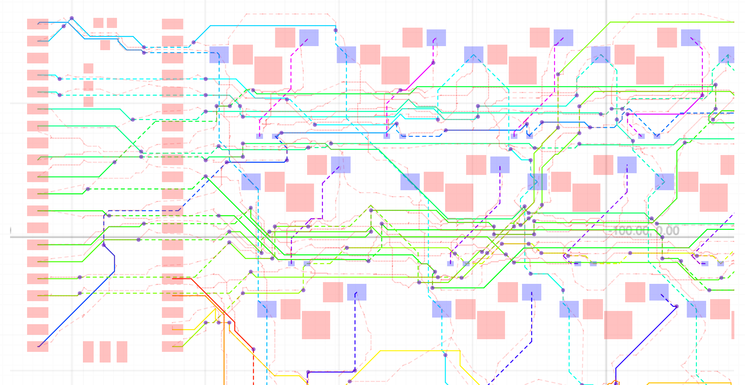
One of my favorite techniques in our autorouter is we run multiple levels of A* to discover the optimal hyperparameters for a particular problem. So we’re basically running each autorouter as a candidate, then using A* to determine which autorouters we should spend the most time on!

See all those numbers at the top? Those are each different configurations of hyper parameters. Running each autorouter fairly would be a huge waste of time- if one autorouter starts to win (it is successfully routing with good costs) allocate more iterations to it! This kind of meta-A* combines a regular cost function that penalizes distance with a cost function that penalizes iterations.

I’m controversially writing our autorouter in Javascript. This is the first thing people call out, but it’s not as unreasonable as you might expect. Consider that when optimizing an algorithm, you’re basically looking at improving two things:

1. Lowering the number of iterations required (make the algorithm smart)

2. Increasing the speed of each iteration

People focus way too much on improving the speed of each iteration. If you are doing something dumb (like converting everything to a grid for overlap testing), Javascript performance will beat you no matter what language you use!

95% of your focus should be on reducing the number of iterations. This is why language doesn’t matter. Whatever gets you to the smartest, most cacheable algorithm fastest is the best language.

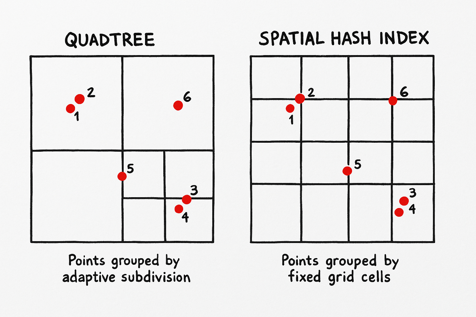
You can’t walk 5 feet into multi-dimensional space optimization without someone mentioning a QuadTree, this incredible data structure that makes O(N) search O(log(N)) when searching for nearby objects in 2d/3d space.

The QuadTree and every general-purpose tree data structure are insanely slow. Trees are not an informed representation of your data.

Why does Javascript use HashSets and HashMaps by default and every chance it gets? They’re super super fast. A Spatial Hash Index is the same concept as a HashMap, but instead of hashing the object we hash it’s location and store it in a Cell (or “bucket of things that are close together”)

Let’s look at how we might replace the QuadTree with a SpatialHashIndex with 20% as much code:

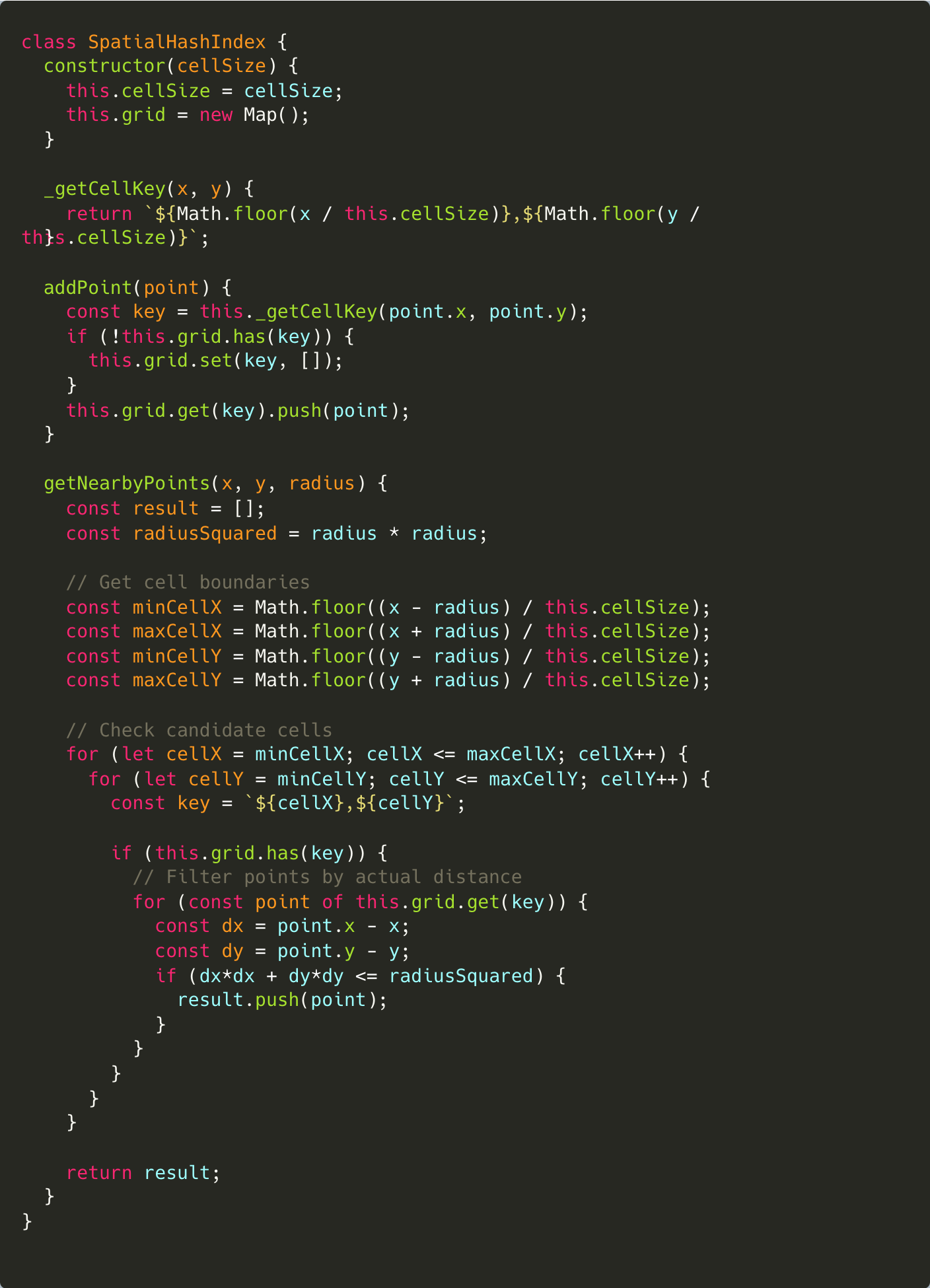
There are many variants of this basic data structure for different types of objects, but they all look pretty similar. We’re basically just creating “buckets” with spatial hashes and filling them with any object that is contained within the cell represented by the spatial hash.

The reason spatial hashes aren’t as popular is you need to be careful about selecting your cell size- this is what makes it an informed algorithm. If your cell size isn’t calibrated well, you’ll end up paying high fixed costs per retrieval. In practice, it’s not that difficult to pick a reasonable cell size.

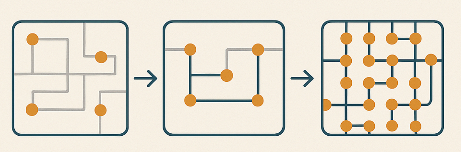
A circuit board like the one inside an IPhone probably has somewhere between 10,000 and 20,000 traces and take a team several months to route with the best EDA tools in world. It can seem daunting to try to optimize such an incredibly complex task- but the truth is the entire industry is neglecting a very simple idea: everything that has been routed has been routed before.

Game developers “pre-bake” navigation meshes into many gigabytes for their games. LLMs compress the entire internet into weights for search. The next generation of autorouters will spatially partition their problems, then call upon a massive cache for pre-solved solutions. The speed of the algorithm doesn’t matter when you have a massive cache with 99% of the autorouting problem pre-solved.

Most algorithms today do not focus on the effective cache-reusability or effective spatial partitioning, but a critical component of future autorouters will be caching inputs and outputs from each stage in a spatially partitioned way.

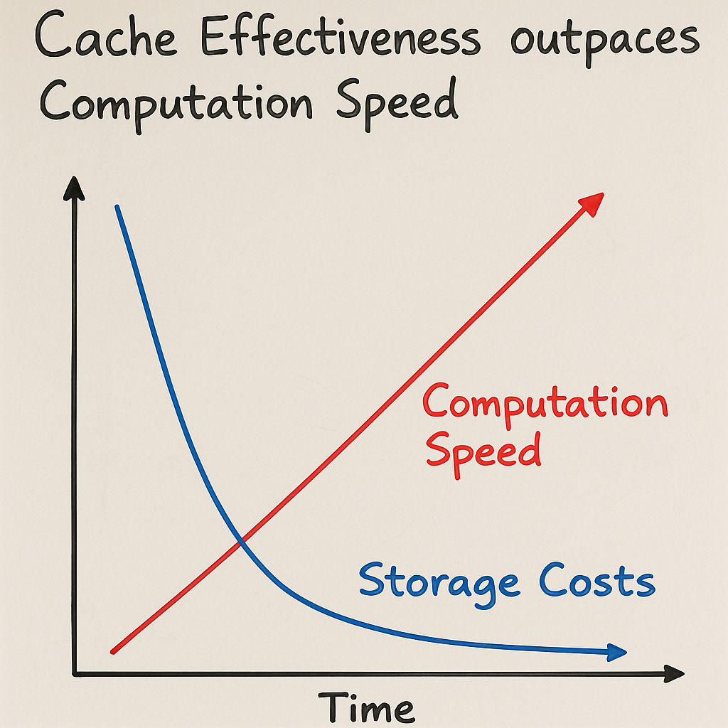
Moreover, the size of storage and caching seems to go down faster than the speed of computation goes up. It’s not a big deal to have a gigabyte cache to make your autorouter 50% faster.

If there is one thing I could have printed on a poster, it would be VISUALIZE THE PROBLEM. You can’t debug problems by staring at numbers.

For every tiny problem we solve, we have a visualization. We will often start with the visualization. Time and time again this enables us to debug and solve problems 10x faster than we could otherwise. Here’s a visualization we made of a subalgorithm for finding 45 degree paths, we use this in our “Path Simplification Phase”, an ~final phase of the autorouter.

Javascript profiling tools are incredibe, you can easily see the exact total time in ms spend on each line of code. You don’t need to use any performance framework, just execute your javascript in the browser and pull up the performance tab. There are also awesome features like flame charts and stuff for memory usage.

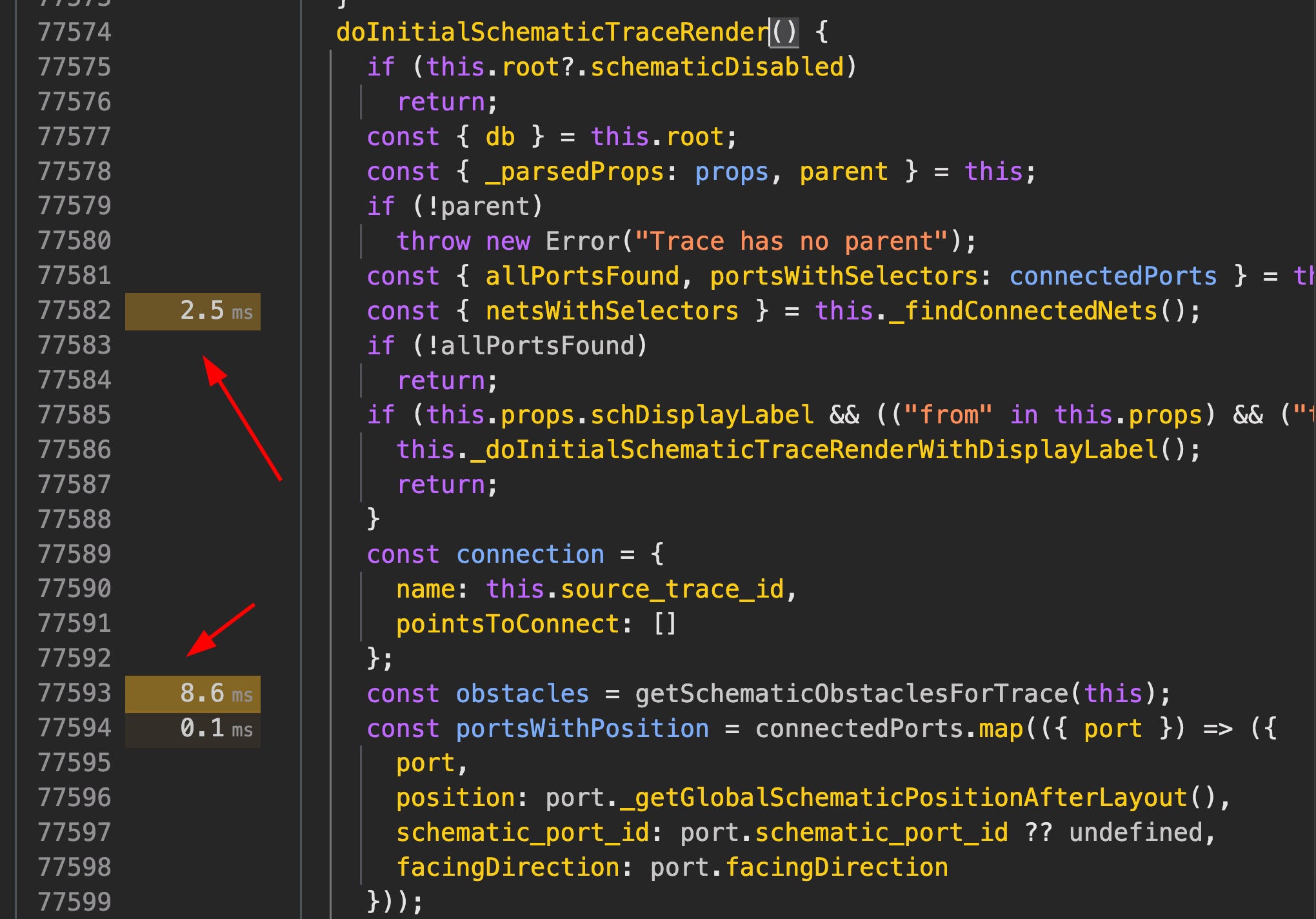
Here’s a little youtube short I made about it

Recursive functions are bad for multiple reasons:

• They are almost always synchronous (can’t be broken out for animation)

• They are inherently a Depth-First Search, and can’t be easily morphed to A*

• You can’t easily track iterations

• Mutability is often unnatural in recursive functions but critical to performance

Here’s an example of an “obviously recursive” function converted to a non-recursive function:

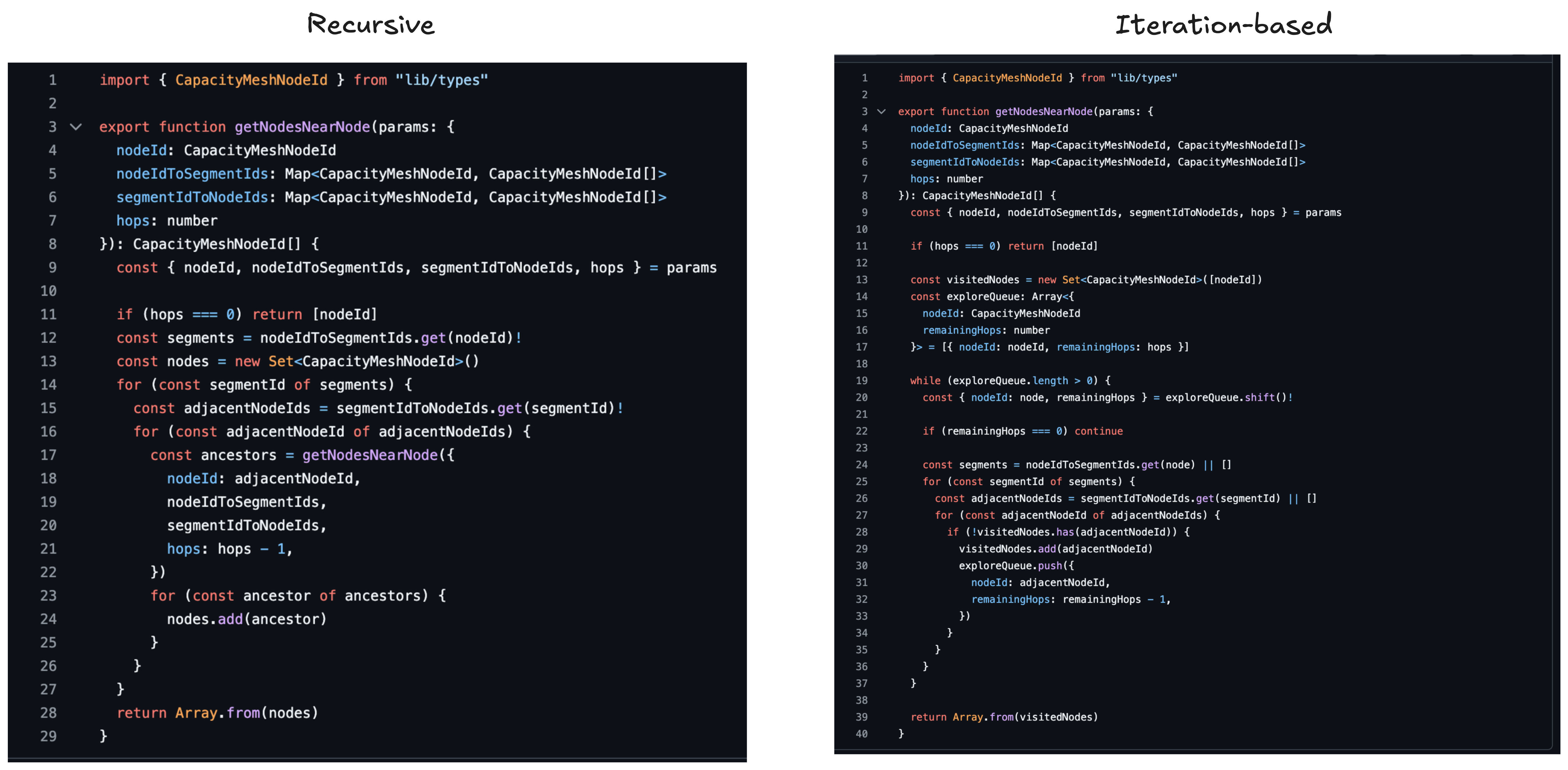
The iteration-based implementation is much faster because it keeps a set of visitedNodes and checks nodes prior to exploration. You can do this with recursive functions, but you have to pass around a mutable object and do other unnatural things. It’s just best to avoid recursive functions when writing performant code.

Monte Carlo algorithms use randomness to iterate towards a solution. They are bad because:

• They lead to non-deterministic, hard-to-debug algorithms

• They are basically never optimal relative to a heuristic

I sometimes use Monte Carlo-style algorithms when I don’t yet know how the algorithm should get to the solution, but I know how to score a candidate. They can help give some basic intuition about how to solve a problem. Once you have something approximating a cost function, do something smarter than Monte Carlo or any other random technique like Simulated Annealing. If your algorithm is sensitive to local minimums, consider using hyper parameters or more complex cost functions. Almost any local minimum your human eye can see can be made into a component of a cost function.

Another way to think about it: How many PCB Designers randomly draw lines on their circuit board? None. Nobody does that. It’s just not a good technique for this domain. You’ll always be able to find a better heuristic.

Our autorouter is currently a pipeline with 13 stages and something like 20 sub-algorithms that we measure the iteration count of for various things like determining spatial partitions or simplifying paths at the boundaries independently autorouted sections.

Being able to overlay different inputs/output visualizations of each stage of the algorithm helps you understand the context surrounding the problem you’re solving. I often ran into issues at downstream stages (often our “high density routing” stage) that could be solved by improving the output of previous stages.

The temptation when building sub-algorithms is to isolate the algorithm to its simplest form, maybe even normalizing around (0, 0). The danger with normalization or any complex transformation is it might impact the ability to quickly see consequences from early stages of the algorithm to later stages of the algorithm. To prevent this, just keep your coordinate space consistent throughout the lifecycle of the algorithm.

Here’s each stage of our algorithm one after another. We often zoom in on this to see what stage is the most guilty culprit for a failed Design Rule Check.

Remember how it’s super important to lower your iteration count?

Animating the iterations of your algorithm will show you how “dumb” it’s being by giving you an intuition for how many iterations are wasted exploring paths that don’t matter. This is particularly helpful when adjusting the greedy multiplier (discussed in 12)

This video is an animation of a simple trace failing to solve, but instead of failing outright attempting to solve endlessly outward. Without the animation, it would have been hard to tell what was going on!

Consider two ways to determine if a trace A overlaps another trace B:

1. Consider each segment of A and B, and check for intersections

2. Create a binary grid that marks each square where trace B is present, then check all the squares where trace A is present to see if B is there

Believe it or not, most people would choose to use Option 2 with a binary grid check, even though this can easily be 1000x slower. People do this because math is hard 🤦

Luckily LLMs make this kind of intersection math trivial. Use fast vector math!! Checking a SINGLE grid square (memory access!) can literally be slower than doing a dot product to determine if two segments intersect!

When doing spatial partitioning of the problem, you can measure the probability of solve failure of each stage with some leading indicators. For example, in the Unravel Autorouter we track the probability of failure for each “Capacity Node” at each major pipeline stage. Each stage focuses on reconfiguring adjacent nodes or rerouting to reduce the probability of failure.

The great thing about probability of failure as a metric is you can literally measure it and improve your prediction as your algorithm changes. Each stage can then do it’s best to minimize the chance of future stages failing.

I think generally prioritizing solvability is better than trying to incorporate too many constraints. Once a board is solved, it’s often easier to “work with that solution” than to generate optimal solution from scratch.

Ok it’s not exactly a secret, maybe a “well-known secret”, but if you don’t know about it, you’re not using A* properly.

By default, A* is guaranteed to give you the optimal solution, but what if you care more about speed than about optimality? Make one tiny change to your f(n)and you have Weighted A*, a variant of A* that solves more greedily, and generally much, much faster!

You can read more about weighted A* and other A* variants here.

Game developers have a lot of the same problems as autorouting developers, so it’s not a bad idea to look for game development papers if you’re searching for related work!

If this was interesting to you, I’d love to show you our autorouter as it gets closer to release. I believe that solving autorouting will be a massive unlock for physical-world innovation and is a key piece to enable the “vibe-building” of electronics. All of our work is MIT-licensed open-source. You can also follow me on twitter.

Keep your files stored safely and securely with the SanDisk 2TB Extreme Portable SSD. With over 69,505 ratings and an impressive 4.6 out of 5 stars, this product has been purchased over 8K+ times in the past month. At only $129.99, this Amazon’s Choice product is a must-have for secure file storage.

Help keep private content private with the included password protection featuring 256-bit AES hardware encryption. Order now for just $129.99 on Amazon!

Help Power Techcratic’s Future – Scan To Support

If Techcratic’s content and insights have helped you, consider giving back by supporting the platform with crypto. Every contribution makes a difference, whether it’s for high-quality content, server maintenance, or future updates. Techcratic is constantly evolving, and your support helps drive that progress.

As a solo operator who wears all the hats, creating content, managing the tech, and running the site, your support allows me to stay focused on delivering valuable resources. Your support keeps everything running smoothly and enables me to continue creating the content you love. I’m deeply grateful for your support, it truly means the world to me! Thank you!